Tutorial: Boostrap and permutation tests

Tutorial: Boostrap and permutation tests#

In this lab we will go over bootstrapping and permutation resampling methods.

Goals:#

Learn to use the boot() function
Learn to write for loops to do permutation tests
Construct a null distribution by permutation as a way of testing hypotheses
Quantify the sampling distribution of a statistic via bootstrapping (construct confidence intervals for your results)

This lab draws from the practice sets at the end of Chapter 5 in James, G., Witten, D., Hastie, T., & Tibshirani, R. (2013). “An introduction to statistical learning: with applications in r.”

A reminder of the difference between bootstrapping and permutation testing#

Both bootstrapping and permutation testing rely on randomization methods. However, their purposes are different, and often confused with each other.

Bootstrapping:

quantifies uncertainty by reusing the data (random resampling with replacement)
answers the question: what is the range of values I can expect for a statistic, given the varaibility in my data?

Permutation testing:

breaks whatever structure may exist between variables of interest while maintaining the structure between others (permute, or shuffle, the relationship between x and y, for example)
allows targeted null hypothesis testing
quantifies the null distribution for a given hypothesis
answers the question: what kind of pattern would you expect to see if there were no statistical relationship between two (or more) variables?

These methods are useful if you need non-parametric estimates of uncertainty for a given statistic (bootstrapping) or if you need a non-parametric way of testing your hypotheses (permutation). In other words, if you don’t want to risk making assumptions about the functional form of your data during uncertainty estimation or hypothesis testing, these randomization methods are for you.

However, keep in mind that there are cons (and assumptions) associated with non-parametric methods. For example, one major limitation of bootstrapping is that you must make the assumption that your data contains variability similar to the kind of variability you might see when you sample new datasets in the wild, given the same statistical model, to make inferential interpretations. See here and here for more information.

Bootstrapping#

First, let’s load the ISLR library to get the Auto dataset, and the boot library so we can use the boot() function.

install.packages("ISLR")
library(ISLR)
library(boot)

Installing package into ‘/usr/local/lib/R/site-library’
(as ‘lib’ is unspecified)

When bootstrapping, we can write our own functions for maximum flexibility. See here for more on writing your own functions in R. We want a function that takes two inputs (a data set and an index of observations) and returns the parameter of interest. In this example, we’ll look at the regression coefficients for the model predicting mpg (miles per gallon) from horsepower.

# The function needs two inputs: Data, Index
boot.fn <- function(data, index){  
    # return: throw this as output
    # coef: extract coefficients from model object 
    return(coef(lm(mpg~horsepower, data=data, subset=index)))}

Let’s test this to make sure it works. We’ll use an index array that takes all 392 observations (rows) in the data set.

print(boot.fn(Auto, 1:392)) # note: "1:392" means all the rows

(Intercept)  horsepower 
 39.9358610  -0.1578447 

Notice this is the same output as when you just run the lm() function with no subset selection (sanity check passed!).

print(coef(lm(mpg~horsepower, data=Auto)))

(Intercept)  horsepower 
 39.9358610  -0.1578447 

Now we can use the boot() function, included in the boot library, to randomly sample with replacement to generate a confidence interval on the regression coefficient. We’ll just test it out with 1000 iterations (set using the R value as an input)

#?boot # uncomment to learn more about the boot() function

boot_obj = boot(Auto ,boot.fn ,R=1000) #R=repetitions 
print(boot_obj) #t1 is the intercept and t2 is the horsepower coeff.

ORDINARY NONPARAMETRIC BOOTSTRAP


Call:
boot(data = Auto, statistic = boot.fn, R = 1000)


Bootstrap Statistics :
      original        bias    std. error
t1* 39.9358610  0.0337235546 0.869718268
t2* -0.1578447 -0.0003595084 0.007482048

attributes(boot_obj) #get all attributes of the boot object 

$names

't0'
't'
'R'
'data'
'seed'
'statistic'
'sim'
'call'
'stype'
'strata'
'weights'

$class

'boot'

$boot_type

'boot'

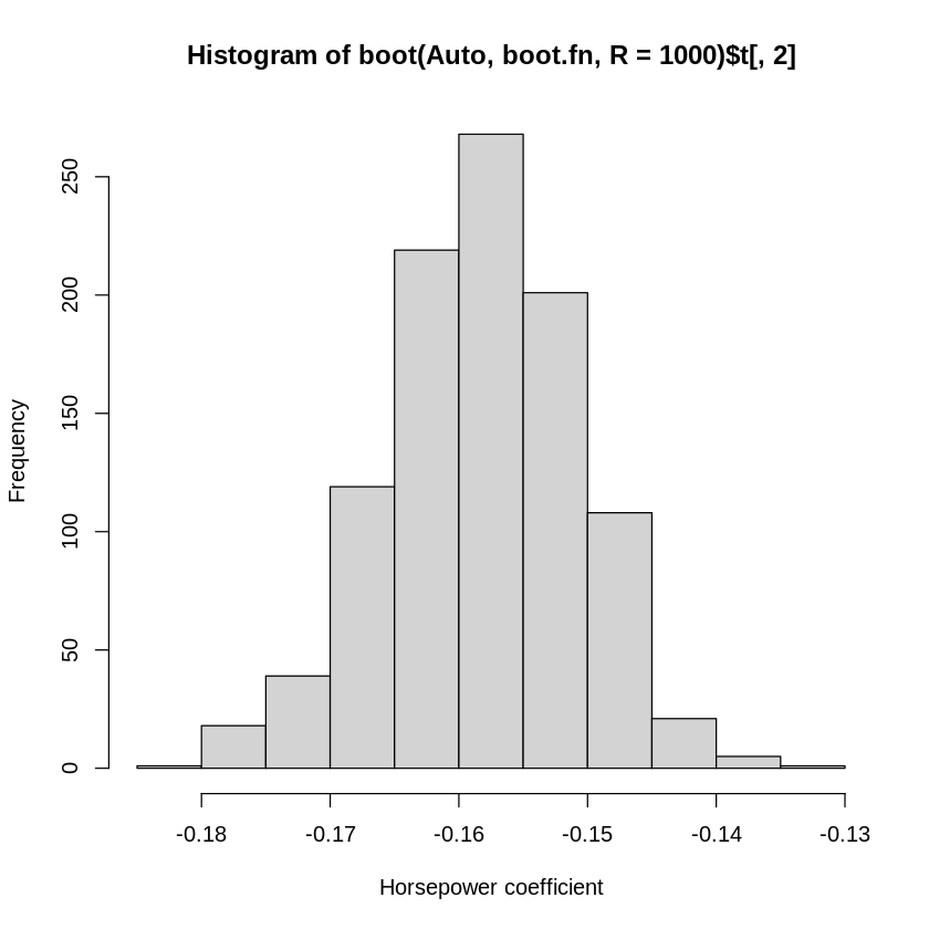
Here the standard error estimate of the two regression coefficients (one for the intercept and one for horsepower) are calculated from the 1000 bootstrapped experiments on the data set. We can see the output from each of the 1000 iterations as well (below we’ll plot just for $\hat{\beta}_{horsepower}$, since that’s more interesting coefficient).

hist(boot(Auto ,boot.fn ,R=1000)$t[,2], xlab="Horsepower coefficient") #we get a distribution of all of the estimates
#                               ^^ indexing the second "t" value

../_images/b2d2f4b64a48b8381a3eb2376cc11ac2c38ef17e8a21a1f68a2b94918f1964d7.png

Now let’s compare these results to the original model where we don’t bootstrap.

# Parametric model
summary(lm(mpg~horsepower ,data=Auto))$coef

A matrix: 2 × 4 of type dbl
	Estimate	Std. Error	t value	Pr(>\|t\|)
(Intercept)	39.9358610	0.717498656	55.65984	1.220362e-187
horsepower	-0.1578447	0.006445501	-24.48914	7.031989e-81

Notice that they produce qualitatively similar results in this case: the parametric estimate and the bootstrapped estimate are both about -0.1578. When the data fit the assumptions of the parametric linear regression model, the bootstrapped estimates will converge to the parametric ones.

Permutation tests#

Remember, that the goal of permutation tests is to use resampling without replacement. By doing this you define the specific null that you want to test and generate a random relationship with which to calculate $P(X|H_0)$. For this we can just use a simple for loop. But first, we need to define what our null is. Here let’s define our null as being that there is no relationship between horsepower and mpg. In other words $$H_0 : \hat{\beta}_{horsepower} = 0$$

If the null is that there is no relationship, then basically the question you’re asking with your analysis is, “Is the relationship between horsepower and mpg stronger than it would be for randomly shuffled pairings of these variables’ observations?”

Note: You are not restricted to these ‘nil’ hypotheses (effect of 0, $\beta$ of 0). The advantage of these kinds of methods is that you can be as flexible as you like in defining your null.

# First let's make a copy of the data set that we'll keep permuting
permAuto = Auto #want to preserve the non-permuted, true form of data!

# Set the number of iterations
R=1000

# Next smake an output object to store the results
perm.coefs=matrix(NA,nrow=R, ncol=2) #filling with nas at first

# Now just write a for loop where we scramble the observations
# in X using the sample() function. We'll scramble the observations in R different ways
for (i in 1:R){
  permAuto$horsepower=Auto$horsepower[sample(392)] # This is a shuffled version of the Auto$horsepower vector
  perm.coefs[i,]=coef(lm(mpg~horsepower, data=permAuto)) # then we get coefficients for linear model of shuffled horsepower to auto
}

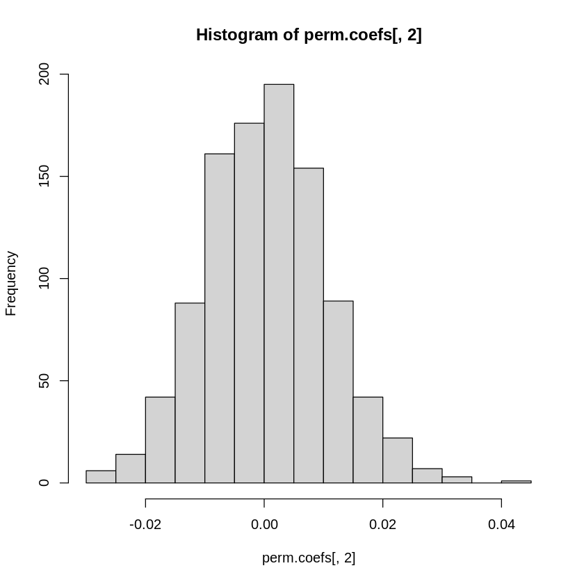
# Take a look at the null distributions
hist(perm.coefs[,2])

../_images/468add280f13754a100db05389b611ca1b0fd1f8a13755027627756796ac7ae5.png

# Now re-estimate the real (unpermuted) effect 
perm.real = coef(lm(mpg~horsepower, data=Auto))
perm.real

(Intercept): 39.9358610211705
horsepower: -0.157844733353654

Notice that the real effect (-0.16) is much larger than the range of coefficient estimates we see for the permuted datasets - it falls outside the range of values in our empirically derived null distribution. But instead of eyeballing it, we can empirically calculate the probability of observing a stronger (i.e., more negative) effect. What is the probability of observing a stronger negative effect than -0.16 due to chance?

#sum the coefficients less than the real coefficient estimate 
#and divide by the number of repetitions to get an empirical probability 
perm.p = sum(perm.coefs[,2]<perm.real[2])/R 
perm.p

0

So we do not see any permuted models that produce results that overlap with the results from the intact model. We can reject the null hypothesis that the $\beta$ estimate for the miles per gallon and horsepower is zero.

Notebook authored by Ven Popov and edited by Krista Bond, Charles Wu, Patience Stevens, and Amy Sentis.