Tutorial: Data as Objects and Tidy Data#
Goals:#
Learn about Tidy Data, long data, and wide data
Learn how to interact with model objects in R, including extracting coefficients
Tidy Data#
When you are working with data frames, it is best practice to keep your data tidy. Tidy data is a very specific term in which the following are true:
Columns are variables
Rows are individual observations
Observation for each variable is stored in the corresponding cell
There are two versions of the tidy data format - long and wide. To illustrate the difference, imagine a repeated measures dataset, where you gather four observations for each subject at four different time points. In the long data format, each row represents an observation at a specific timepoint for a specific subject. Each subject has multiple rows of observations. The columns will be subject, timepoint, and observation. For example:
long_data <- data.frame(subject = rep(1:3, each=4),  # rep repeats a vector n times
                        timepoint = rep(1:4, times=3), # same as previous
                        observation = round(rnorm(12), 2)) #rnorm simulates a normal distribution
long_data # print out long data table
| subject | timepoint | observation |
|---|---|---|
| <int> | <int> | <dbl> |
| 1 | 1 | -1.09 |
| 1 | 2 | 0.10 |
| 1 | 3 | 0.84 |
| 1 | 4 | 1.09 |
| 2 | 1 | -0.81 |
| 2 | 2 | -0.13 |
| 2 | 3 | 0.76 |
| 2 | 4 | -0.44 |
| 3 | 1 | 2.09 |
| 3 | 2 | -1.62 |
| 3 | 3 | 0.95 |
| 3 | 4 | -0.09 |
Alternatively, the data can be organized in a wide format, in which each row is a single subject, the four different timepoints are represented as different columns, and the observation for each timepoint is stored at a cell within that column. Like this (don’t worry about the code for now, it is explained in the next tutorial):
library(tidyverse) #We'll learn about this package in the next tutorial!

long_data  %>% # This is a pipe. We will learn about this later
    mutate(timepoint = paste0('time',timepoint))  %>%  # mutate makes a new column
    spread(timepoint, observation) # spread pushes an observation across multiple columns
| subject | time1 | time2 | time3 | time4 |
|---|---|---|---|---|
| <int> | <dbl> | <dbl> | <dbl> | <dbl> |
| 1 | -1.09 | 0.10 | 0.84 | 1.09 |
| 2 | -0.81 | -0.13 | 0.76 | -0.44 |
| 3 | 2.09 | -1.62 | 0.95 | -0.09 |
Interacting with model objects in R#
Whenever you run a regression or any other type of model, the resulting model is saved in an object with properties you can access. This is handy for fitting a model once, and then referencing different aspects of that model’s performance and fit. Let’s see an example:
# generate data where y is a function of two variables, x1 and x2
x1 <- seq(-4,4,0.5) #generate data ranging from -4 to 4 in steps of 0.5
x2 <- seq(-4,4,0.5)

#specify a sigmoidal relationship between x1 and y
#and a linear relationship between x2 and y
dat <- expand.grid(x1=x1, x2=x2) %>%
    mutate(y = 1/(1+exp(-x1)) + 0.1*x2)

head(dat)
| x1 | x2 | y | |
|---|---|---|---|
| <dbl> | <dbl> | <dbl> | |
| 1 | -4.0 | -4 | -0.3820138 |
| 2 | -3.5 | -4 | -0.3706878 |
| 3 | -3.0 | -4 | -0.3525741 |
| 4 | -2.5 | -4 | -0.3241418 |
| 5 | -2.0 | -4 | -0.2807971 |
| 6 | -1.5 | -4 | -0.2175745 |
Note that expand.grid just creates a data frame with all possible pairs of the input variables. So here, each value of x1 was paired with an x2 value of -4, then with an x2 value of -3.5, etc…
We’ll learn more about the pipe (%>%) and mutate in the next tutorial!
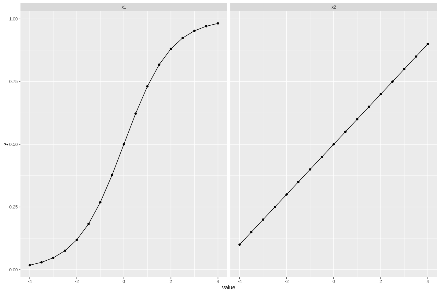
Here is how y depends on x1 and x2:
# setting figure size
options(repr.plot.width=12, repr.plot.height=8)

dat  %>%
    gather(var, value, x1, x2) %>% # make it long format - only x1 or x2 in each row
    ggplot(aes(value, y)) + # we will learn aboug ggplot in a later tutorial
    stat_summary(geom='point',fun=mean) +
    stat_summary(geom='line',fun=mean) +
    facet_wrap(~var) # optimally wraps figures as needed
Now, let’s add some noise and try to fit a regression model
#create new y_obs variable with normally distributed noise
dat <- mutate(dat, y_obs = y + rnorm(length(y), mean=0, sd=0.1))

#fit a linear model to find the regression coefficients
model_fit <- lm(y_obs ~ x1 + x2, data=dat)
The resulting model is saved in the model_fit variable. This is the “model object”, and you can do a number of things with it. First, the str() command, which is a general function for printing the structure of r objects, will tell you what you can find in the model object. As you can see below, it is a list of different variables, which you can access by typing the name of the model, followed by $variable.
str(model_fit) #print the structure of the model object
List of 12
 $ coefficients : Named num [1:3] 0.4996 0.1507 0.0999
  ..- attr(*, "names")= chr [1:3] "(Intercept)" "x1" "x2"
 $ residuals    : Named num [1:289] 0.0767 0.1405 0.0611 -0.0984 -0.0678 ...
  ..- attr(*, "names")= chr [1:289] "1" "2" "3" "4" ...
 $ effects      : Named num [1:289] -8.4925 6.2743 4.1608 -0.1134 -0.0814 ...
  ..- attr(*, "names")= chr [1:289] "(Intercept)" "x1" "x2" "" ...
 $ rank         : int 3
 $ fitted.values: Named num [1:289] -0.503 -0.427 -0.352 -0.277 -0.201 ...
  ..- attr(*, "names")= chr [1:289] "1" "2" "3" "4" ...
 $ assign       : int [1:3] 0 1 2
 $ qr           :List of 5
  ..$ qr   : num [1:289, 1:3] -17 0.0588 0.0588 0.0588 0.0588 ...
  .. ..- attr(*, "dimnames")=List of 2
  .. .. ..$ : chr [1:289] "1" "2" "3" "4" ...
  .. .. ..$ : chr [1:3] "(Intercept)" "x1" "x2"
  .. ..- attr(*, "assign")= int [1:3] 0 1 2
  ..$ qraux: num [1:3] 1.06 1.08 1.09
  ..$ pivot: int [1:3] 1 2 3
  ..$ tol  : num 1e-07
  ..$ rank : int 3
  ..- attr(*, "class")= chr "qr"
 $ df.residual  : int 286
 $ xlevels      : Named list()
 $ call         : language lm(formula = y_obs ~ x1 + x2, data = dat)
 $ terms        :Classes 'terms', 'formula'  language y_obs ~ x1 + x2
  .. ..- attr(*, "variables")= language list(y_obs, x1, x2)
  .. ..- attr(*, "factors")= int [1:3, 1:2] 0 1 0 0 0 1
  .. .. ..- attr(*, "dimnames")=List of 2
  .. .. .. ..$ : chr [1:3] "y_obs" "x1" "x2"
  .. .. .. ..$ : chr [1:2] "x1" "x2"
  .. ..- attr(*, "term.labels")= chr [1:2] "x1" "x2"
  .. ..- attr(*, "order")= int [1:2] 1 1
  .. ..- attr(*, "intercept")= int 1
  .. ..- attr(*, "response")= int 1
  .. ..- attr(*, ".Environment")=<environment: R_GlobalEnv>
  .. ..- attr(*, "predvars")= language list(y_obs, x1, x2)
  .. ..- attr(*, "dataClasses")= Named chr [1:3] "numeric" "numeric" "numeric"
  .. .. ..- attr(*, "names")= chr [1:3] "y_obs" "x1" "x2"
 $ model        :'data.frame':	289 obs. of  3 variables:
  ..$ y_obs: num [1:289] -0.426 -0.287 -0.291 -0.375 -0.269 ...
  ..$ x1   : num [1:289] -4 -3.5 -3 -2.5 -2 -1.5 -1 -0.5 0 0.5 ...
  ..$ x2   : num [1:289] -4 -4 -4 -4 -4 -4 -4 -4 -4 -4 ...
  ..- attr(*, "terms")=Classes 'terms', 'formula'  language y_obs ~ x1 + x2
  .. .. ..- attr(*, "variables")= language list(y_obs, x1, x2)
  .. .. ..- attr(*, "factors")= int [1:3, 1:2] 0 1 0 0 0 1
  .. .. .. ..- attr(*, "dimnames")=List of 2
  .. .. .. .. ..$ : chr [1:3] "y_obs" "x1" "x2"
  .. .. .. .. ..$ : chr [1:2] "x1" "x2"
  .. .. ..- attr(*, "term.labels")= chr [1:2] "x1" "x2"
  .. .. ..- attr(*, "order")= int [1:2] 1 1
  .. .. ..- attr(*, "intercept")= int 1
  .. .. ..- attr(*, "response")= int 1
  .. .. ..- attr(*, ".Environment")=<environment: R_GlobalEnv>
  .. .. ..- attr(*, "predvars")= language list(y_obs, x1, x2)
  .. .. ..- attr(*, "dataClasses")= Named chr [1:3] "numeric" "numeric" "numeric"
  .. .. .. ..- attr(*, "names")= chr [1:3] "y_obs" "x1" "x2"
 - attr(*, "class")= chr "lm"
For example, if we want to extract the estimated regression coefficients, we can type this, which returns a named vector.
model_fit$coefficients
- (Intercept)
- 0.499559922079091
- x1
- 0.150675486478537
- x2
- 0.0999191218958173
If we run multiple models, we might want to store these values in a data.frame, rather than a named vector like this:
#store the coefficients in a variable
coef <- model_fit$coefficients

#save the name/value of the coefficients in a dataframe
data.frame(name = names(coef), value = coef)
| name | value | |
|---|---|---|
| <chr> | <dbl> | |
| (Intercept) | (Intercept) | 0.49955992 |
| x1 | x1 | 0.15067549 |
| x2 | x2 | 0.09991912 |
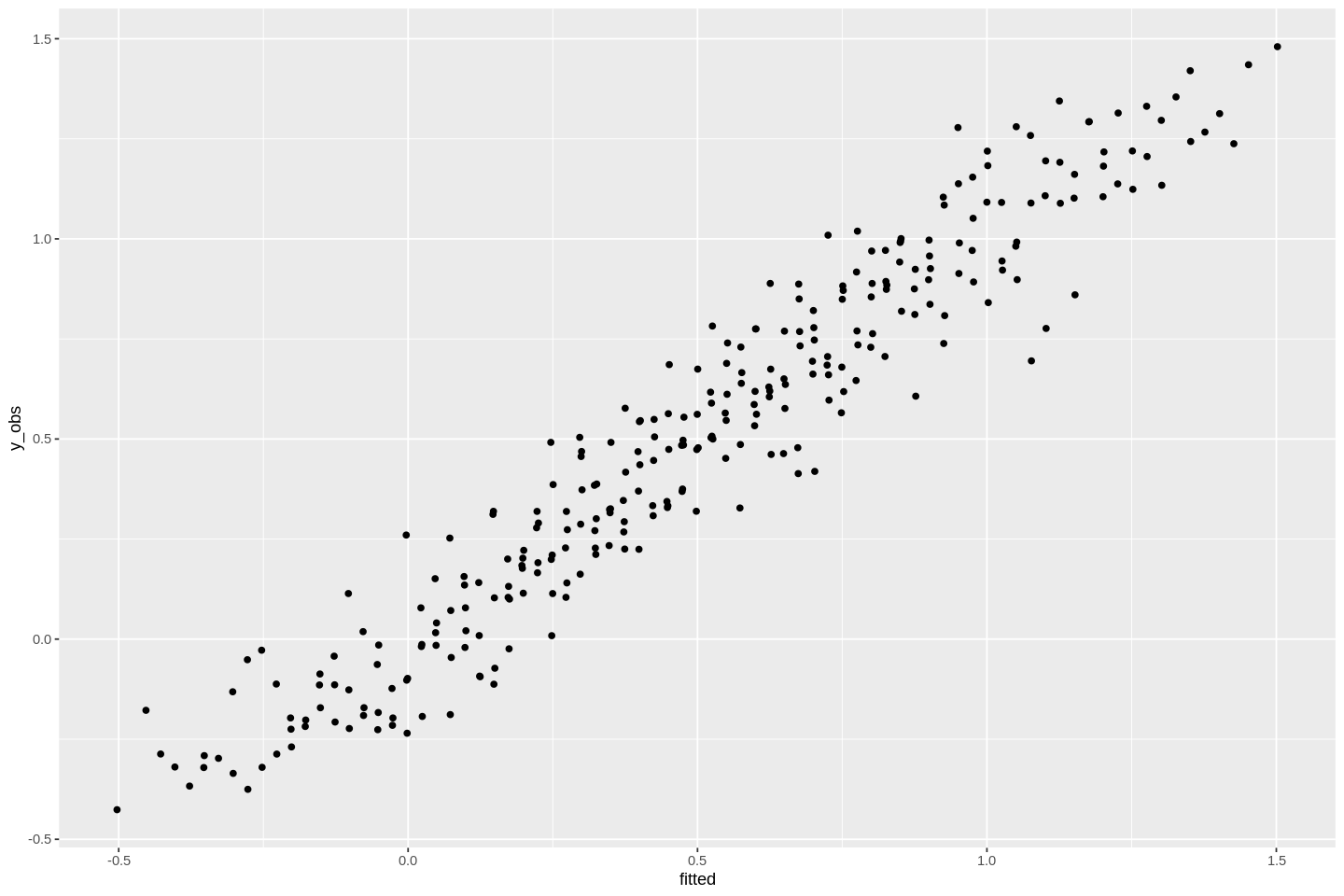
You can also extract the prediction of the model. They are stored under $fitted.values, or you can get them by typing fitted(model_fit), which returns the same values. Then, we can plot the observed values against the predicted values:
#extract model estimate of y for each x and store in df as fitted
dat$fitted <- model_fit$fitted.values

head(dat) #we see "fitted" column added
| x1 | x2 | y | y_obs | fitted | |
|---|---|---|---|---|---|
| <dbl> | <dbl> | <dbl> | <dbl> | <dbl> | |
| 1 | -4.0 | -4 | -0.3820138 | -0.4261378 | -0.5028185 |
| 2 | -3.5 | -4 | -0.3706878 | -0.2869985 | -0.4274808 |
| 3 | -3.0 | -4 | -0.3525741 | -0.2910417 | -0.3521430 |
| 4 | -2.5 | -4 | -0.3241418 | -0.3752198 | -0.2768053 |
| 5 | -2.0 | -4 | -0.2807971 | -0.2692938 | -0.2014675 |
| 6 | -1.5 | -4 | -0.2175745 | -0.2070880 | -0.1261298 |
#plot fitted against the observed data
ggplot(dat, aes(fitted, y_obs)) +
    stat_summary(geom='point',fun=mean)
Given your fitted model, you can also easily generate predictions of y given new values of x using the predict function:
new_data <- data.frame(x1=-5, x2=10) #new x-values to give to the model
predict(model_fit, newdata = new_data) #predict the y value for a given x
That’s all for now! We’ll dive into some more advanced functions for data manipulation in R in the next tutorial.
Notebook authored by Ven Popov and edited by Krista Bond, Charles Wu, Patience Stevens, Amy Sentis, and Fiona Horner.


